
Hydraulics represents one of the most important branches of fluid mechanics, dealing with the behavior of liquids in motion and at rest. The study of hydraulic systems encompasses the analysis of flow states, motion laws, energy conversion, and the interaction forces between flowing liquids and solid boundaries.
When engineers and technicians ask "what are the principles of hydraulics," they are essentially inquiring about three fundamental equations that form the backbone of hydraulic theory: the continuity equation, Bernoulli's equation, and the momentum equation. These principles not only constitute the foundation of fluid dynamics but also serve as the theoretical basis for problem analysis and design calculations in hydraulic technology.
Hydraulic systems utilize the principles of fluid mechanics to transmit power efficiently in various industrial applications.
The study of fluid flow necessarily involves considering the effects of viscosity. However, due to the extreme complexity of this problem, engineers often begin their analysis by assuming that the fluid has no viscosity, then subsequently consider viscous effects and validate or modify ideal conclusions through experimental methods. This same approach can be applied to handle fluid compressibility issues. Generally, a hypothetical fluid that is both inviscid and incompressible is referred to as an ideal fluid.
Understanding what are the principles of hydraulics requires recognizing that real fluids always exhibit some degree of viscosity and compressibility, but the ideal fluid concept provides a valuable starting point for analysis. This simplification allows engineers to develop fundamental equations that can later be modified with correction factors based on experimental data.
When fluid flows through a system, if the pressure, velocity, and density at any point in the fluid do not change with time, this type of flow is called steady flow (also known as stationary flow or time-invariant flow). Conversely, if any of these parameters—pressure, velocity, or density—varies with time, the flow is termed unsteady flow (also called non-stationary flow or time-variant flow).
In practical hydraulic systems, achieving perfectly steady flow is challenging, but many industrial applications can be approximated as steady flow for design purposes. This approximation significantly simplifies the mathematical analysis while still providing sufficiently accurate results for engineering applications.
Fluid flow can be categorized based on its dimensional characteristics. When fluid moves entirely in a linear fashion, it is called one-dimensional flow. When it exhibits planar or spatial motion, it is referred to as two-dimensional or three-dimensional flow, respectively. One-dimensional flow represents the simplest case for analysis.
In the strictest sense, one-dimensional flow requires that the velocity vectors at all points across a flow cross-section be completely identical, with the motion parameters being functions of a single coordinate. Such conditions are extremely rare in reality. However, engineers commonly analyze fluid flow in enclosed containers as one-dimensional flow, then apply experimental corrections to the calculated results.
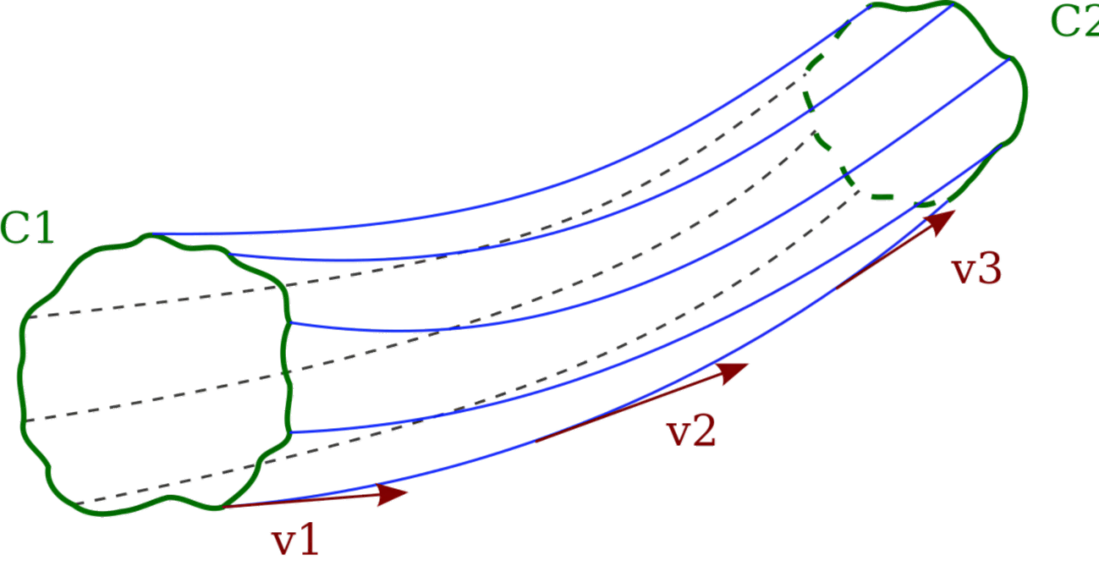
A streamline is a curve that indicates the instantaneous motion state of fluid particles at a given moment. At any point along a streamline, the instantaneous flow direction coincides with the tangent to the streamline at that point. Since each point in the fluid has only one velocity at any instant, streamlines can neither intersect nor exhibit sharp turns—they must be smooth curves.
When a closed curve is drawn within a flow field, all streamlines passing through this curve form a tubular surface called a stream tube. The collection of all streamlines within a stream tube is called a stream bundle. According to the property that streamlines cannot intersect, fluid particles inside and outside a stream tube cannot cross the stream tube surface.
The cross-section perpendicular to a stream bundle is called the flow cross-section (or flow area). The velocity at each point on a flow cross-section is perpendicular to it. Therefore, a flow cross-section may be either planar or curved. A stream bundle with an infinitesimally small flow area is called an elementary stream bundle.
Streamlines show the direction of fluid flow at any given moment and never intersect, providing valuable insights into flow behavior.
The volume of fluid passing through a given flow cross-section per unit time is called the volume flow rate (unless otherwise specified, flow rate in hydraulic systems refers to volume flow rate). Flow rate is denoted by q and is measured in m³/s or L/min.
When fluid flows through a differential flow cross-section dA, the velocity u at all points on this section can be considered equal. Therefore, the flow rate through this differential section is dq = u·dA. The total flow rate through the entire cross-section A is:
For real fluid flow, due to viscous forces, the velocity u varies across the flow cross-section, and its distribution pattern is often unknown. This makes calculating flow rate using integration inconvenient. To address this challenge, engineers introduced the concept of average velocity.
The average velocity assumes uniform velocity distribution across the flow cross-section, where the flow rate at this uniform velocity v equals the actual flow rate. This gives us:
From this, the average velocity across the flow cross-section is:
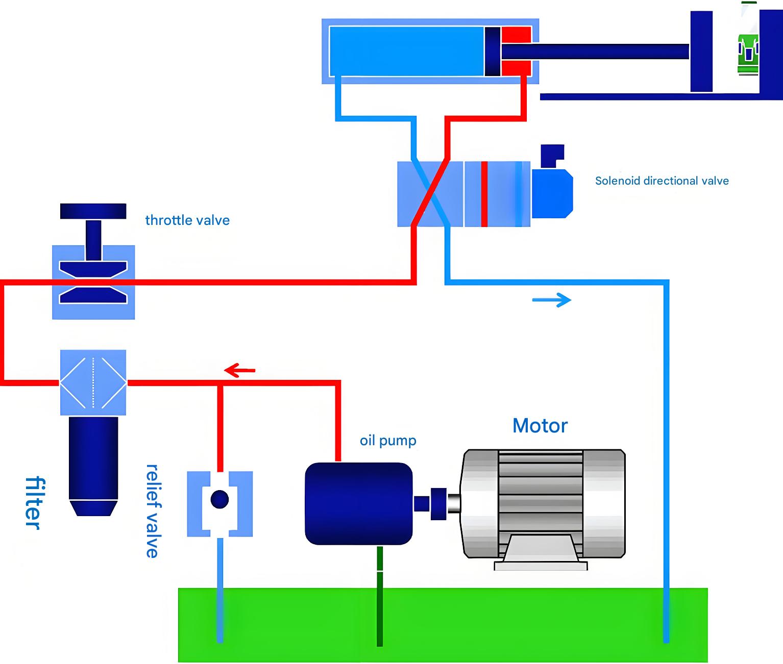
In practical engineering applications, average velocity v has significant utility. For instance, when a hydraulic cylinder operates, the piston's velocity equals the average velocity of the fluid within the cylinder. This establishes the relationship between piston velocity v, the cylinder's effective area A, and flow rate q. When the hydraulic cylinder's effective area is fixed, piston velocity depends on the fluid flow rate delivered to the cylinder.
Actual velocity profile vs. average velocity approximation in pipe flow
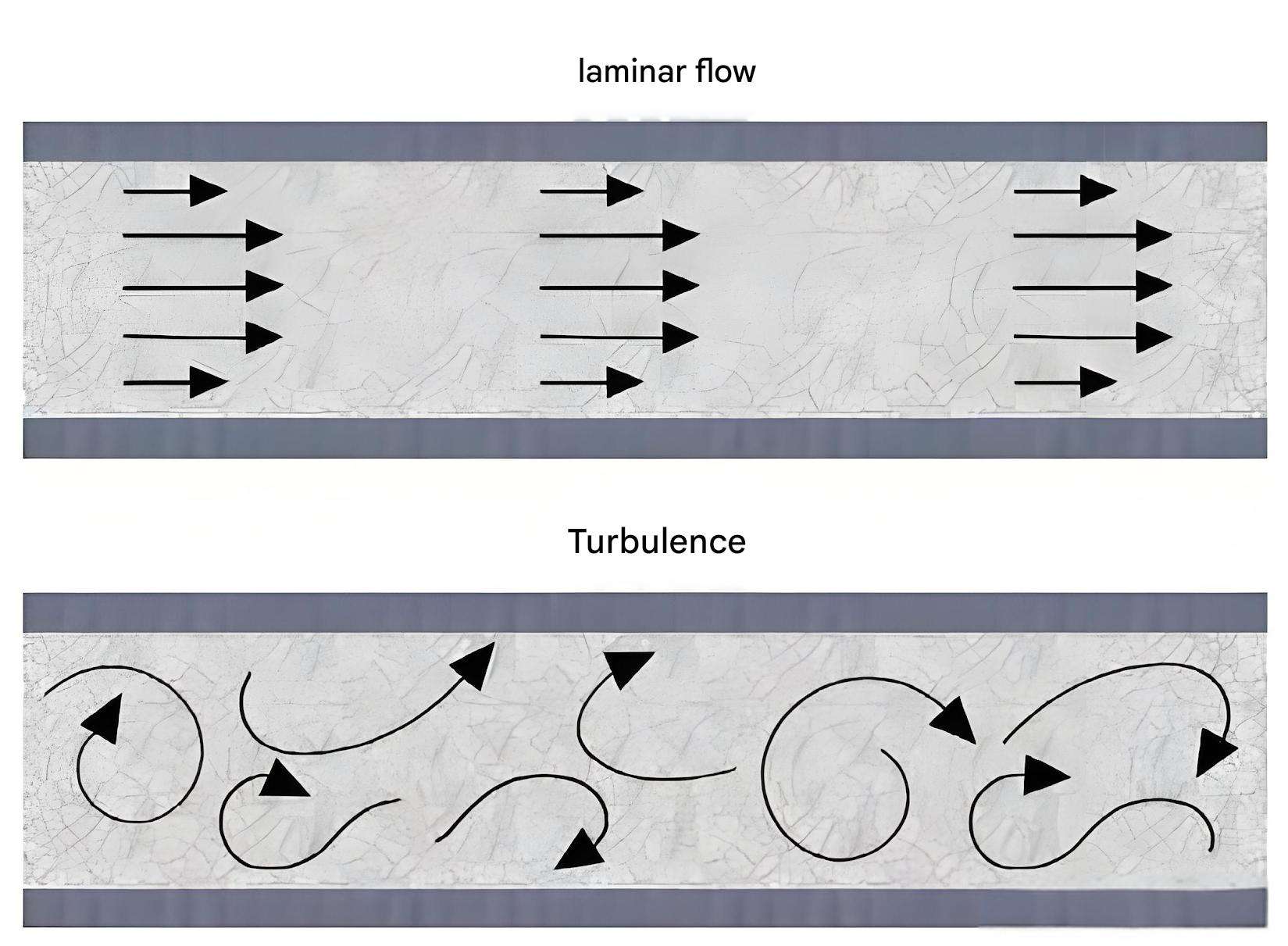
Fluid flow exhibits two distinct states: laminar and turbulent flow. These flow regimes can be observed through Reynolds' classic experiment. Understanding what are the principles of hydraulics fundamentally requires comprehending these flow states and their transitions.
The Reynolds experiment apparatus consists of a water tank maintained at constant height through continuous water supply. A container with colored water releases dye through a fine tube into a horizontal glass pipe. By adjusting a valve, the flow velocity in the glass pipe can be controlled. At low velocities, the colored water forms a distinct straight line in the glass pipe, unmixed with the clear water. This indicates that the fluid flows in layers without mutual interference—a state called laminar flow.
As the valve is opened to increase flow velocity, at a certain point, the colored line begins to oscillate and form waves, indicating the breakdown of laminar flow. With further velocity increase, the colored water completely mixes with the clear water, and the distinct line disappears entirely, indicating fully turbulent flow.
Experiments demonstrate that flow regime in circular pipes depends not only on average velocity v but also on pipe diameter d and kinematic viscosity ν. The dimensionless parameter combining these three variables is the Reynolds number:
The Reynolds number is dimensionless, meaning that for pipes with the same cross-section, identical Reynolds numbers indicate identical flow states. The critical Reynolds number (Re_c) marks the transition between flow regimes. When the actual Reynolds number is less than the critical value, flow is laminar; otherwise, it is turbulent. Critical Reynolds numbers for common pipe configurations are determined experimentally and tabulated for reference.
The Reynolds number represents the dimensionless ratio of inertial forces to viscous forces in the fluid. When the Reynolds number is large, inertial forces dominate, and the fluid exhibits turbulent behavior. When the Reynolds number is small, viscous forces dominate, resulting in laminar flow.
For non-circular cross-sections, the Reynolds number calculation uses the hydraulic diameter:
Where the hydraulic diameter is:
Here, A represents the flow cross-sectional area, and χ is the wetted perimeter—the length of the cross-section boundary in contact with the fluid. The hydraulic diameter reflects the pipe's flow capacity: a larger hydraulic diameter indicates shorter contact between fluid and pipe walls, resulting in lower wall resistance and greater flow capacity.
The continuity equation represents the application of mass conservation law in fluid mechanics. This fundamental principle is essential for anyone seeking to understand what are the principles of hydraulics in practical applications.
Consider fluid flowing steadily through a pipe system. Taking two arbitrary cross-sections labeled 1 and 2, with areas A₁ and A₂ respectively, and fluid densities and average velocities at these sections being ρ₁, v₁ and ρ₂, v₂ respectively. According to mass conservation, the mass flow rate through both sections must be equal:
When fluid compressibility is negligible (ρ₁ = ρ₂), this simplifies to:
Or written as: q = vA = constant
This equation leads to an important conclusion: for ideal fluid flowing steadily in a closed conduit, regardless of how the average velocity and cross-sectional area vary along the flow path, the flow rate through each cross-section remains constant. This principle has profound implications for hydraulic system design, particularly in determining pipe sizes and predicting flow velocities at different points in the system.
The continuity equation helps engineers size components properly, ensuring that flow requirements are met throughout the hydraulic circuit. It also explains why fluid velocity increases when passing through restrictions and decreases in expanded sections, a principle utilized in various hydraulic devices such as venturi meters and jet pumps.
Bernoulli's equation represents the application of energy conservation law in fluid mechanics. This equation is perhaps the most frequently applied principle when engineers investigate what are the principles of hydraulics for system design and analysis.
Consider ideal fluid flowing steadily through a pipe. Taking a differential stream bundle ab as the subject of analysis, let the heights of sections a and b from a reference plane O-O be h₁ and h₂ respectively, with cross-sectional areas dA₁ and dA₂, pressures p₁ and p₂, and velocities u₁ and u₂.
During an infinitesimal time interval dt, fluid at section a moves to a', while fluid at section b moves to b'. Analyzing the energy changes in this fluid segment:
For ideal fluid without viscosity, no internal friction exists, so work done by external forces equals the algebraic sum of work done by pressure at both sections:
Using the continuity equation dA₁u₁ = dA₂u₂ = dq:
According to energy conservation, work done by external forces equals the change in mechanical energy (ΔE = W), yielding:
Each term in Bernoulli's equation has specific physical meaning:
The equation states that for ideal fluid flowing steadily in a closed conduit, three forms of energy exist: pressure energy, kinetic energy, and potential energy. These can transform into one another, but at any position in the pipe, the total energy per unit mass remains constant.
Real fluids possess viscosity, causing friction that dissipates energy. Additionally, changes in pipe geometry create flow disturbances that consume energy. Therefore, real fluid flow involves energy losses, denoted as h_w·g per unit mass.
Furthermore, since velocity distribution across a real flow cross-section is non-uniform, using average velocity to calculate kinetic energy introduces error. This is corrected by introducing a kinetic energy correction coefficient α.
The modified Bernoulli equation for real fluid becomes:
Or alternatively:
The kinetic energy correction coefficients α₁ and α₂ depend on flow regime: α = 1 for turbulent flow and α = 2 for laminar flow.
Bernoulli's equation illustrates how pressure energy, kinetic energy, and potential energy transform between each other while conserving total energy (minus losses in real systems).
The momentum equation represents the specific application of momentum theorem in fluid mechanics. In hydraulic systems, when calculating forces exerted by fluid flow on solid boundaries, the momentum equation provides a convenient solution method. This is another crucial aspect when exploring what are the principles of hydraulics for force analysis.
Classical mechanics momentum theorem states that external force acting on an object equals the rate of change of momentum:
For steadily flowing fluid, neglecting compressibility, substituting m = ρq·dt and introducing momentum correction coefficient β to account for using average velocity instead of actual velocity distribution:
Where:
Equation 2-24 is a vector equation. In practice, vectors must be decomposed into components along specified directions. For example, the momentum equation in the x-direction:
Engineering problems often require determining fluid forces on channel walls—the reaction force F' to F in the momentum equation, called steady-state hydraulic force. The x-direction steady-state hydraulic force is:
This equation is invaluable for calculating forces in hydraulic components such as valves, bends, and nozzles, where fluid momentum changes significantly.
Understanding what are the principles of hydraulics involves recognizing how the three fundamental equations—continuity, Bernoulli's, and momentum—work together in real systems. These equations are rarely used in isolation; instead, they complement each other in solving complex hydraulic problems.
For instance, when designing a hydraulic cylinder system, the continuity equation determines flow requirements, Bernoulli's equation analyzes pressure distributions and energy losses, while the momentum equation calculates forces on components. This integrated approach ensures comprehensive system analysis and optimal design.
Real hydraulic systems experience two primary types of energy losses:
Accurate prediction of these losses is crucial for system efficiency and performance. Engineers use empirical correlations and experimental data to estimate losses, incorporating them into modified forms of the fundamental equations.
The principles discussed enable various flow measurement methods:
Utilize Bernoulli's equation to relate pressure drop to flow rate. Examples include orifice plates, Venturi meters, and flow nozzles.
Apply continuity equation to convert point velocities to volume flow rates. Examples include Pitot tubes, turbine meters, and electromagnetic flow meters.
Employ momentum equation to relate fluid forces to flow rate. Examples include impact meters and vortex shedding flow meters.
Each technique has advantages and limitations, with selection depending on accuracy requirements, fluid properties, and operating conditions.
While this discussion primarily addresses Newtonian fluids (where viscosity is independent of shear rate), many industrial hydraulic fluids exhibit non-Newtonian behavior. Understanding what are the principles of hydraulics for these fluids requires modified equations accounting for variable viscosity.
Common non-Newtonian behaviors in hydraulic fluids include:
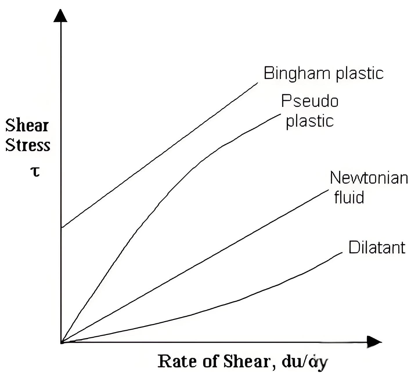
Different fluid types exhibit varying relationships between shear stress and shear rate, requiring specialized analysis techniques.
Temperature significantly influences hydraulic fluid properties, particularly viscosity and density. As temperature increases, viscosity typically decreases exponentially, affecting Reynolds number and flow regime. This temperature dependence must be considered in systems operating over wide temperature ranges.
Temperature variations also cause thermal expansion of both fluid and system components, potentially affecting clearances, seal performance, and volumetric efficiency. Proper thermal management ensures consistent system performance across operating conditions.
Although often neglected in basic analysis, fluid compressibility becomes important in certain situations:
The bulk modulus characterizes fluid compressibility, relating pressure changes to volume changes. Including compressibility effects requires modified equations incorporating density variations.
Cavitation occurs when local pressure drops below vapor pressure, causing vapor bubble formation. These bubbles violently collapse when entering higher-pressure regions, causing noise, vibration, and component damage. Understanding cavitation is essential for proper system design, particularly for pumps and valves.
Preventing cavitation involves:
Applying hydraulic principles to component selection ensures optimal system performance. Key considerations include:
Maximizing hydraulic system efficiency requires understanding energy transformation and loss mechanisms. Engineers asking what are the principles of hydraulics for efficiency improvement focus on:
Dynamic system behavior involves time-varying flows and pressures, requiring extended analysis beyond steady-state equations. Key dynamic considerations include:
Contamination significantly impacts hydraulic system performance and reliability. Particles cause wear, stick valves, and clog orifices. Understanding flow patterns helps design effective filtration strategies:
Modern hydraulic system design increasingly relies on computational methods to solve complex flow problems. These techniques build upon fundamental principles while handling realistic geometries and conditions:
Discretizes flow domain into elements, solving governing equations at nodes. Particularly useful for structural-fluid interaction problems.
Conserves quantities over control volumes, naturally satisfying continuity. Widely used in computational fluid dynamics (CFD) software.
Approximates derivatives using discrete points, simple to implement for regular geometries.
Commercial software packages implement these numerical methods, allowing engineers to analyze complex hydraulic systems without extensive programming. When investigating what are the principles of hydraulics through simulation, engineers can:
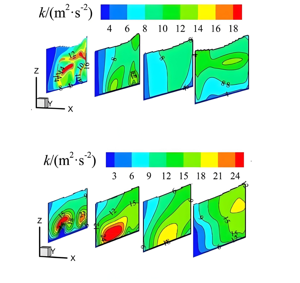
Computational fluid dynamics software visualizes complex flow patterns that would be difficult to analyze with theoretical methods alone.
Computational results require validation against experimental data or analytical solutions. Key validation steps include:
Experimental investigation remains crucial for understanding hydraulic phenomena and validating theoretical predictions. Standard laboratory equipment includes:
When full-scale testing is impractical, scaled models provide valuable insights. Dimensional analysis ensures similar flow behavior between model and prototype:
Reynolds number matching ensures similar flow regimes between model and prototype, though complete similarity is often impossible, requiring careful interpretation of results.
Real-world hydraulic systems require field testing to verify performance and diagnose problems. Understanding what are the principles of hydraulics guides systematic troubleshooting:
Integration of sensors, actuators, and control systems creates intelligent hydraulic systems with enhanced capabilities:
Integration of sensors and digital controls enables real-time monitoring and optimization of hydraulic systems.
New materials enhance hydraulic system performance:
Environmental concerns drive development of eco-friendly hydraulic technologies:
Virtual replicas of physical hydraulic systems enable:
Understanding what are the principles of hydraulics becomes even more critical as these digital models require accurate physical foundations.
The principles of hydraulics—embodied in the continuity equation, Bernoulli's equation, and momentum equation—provide the theoretical foundation for understanding and designing fluid power systems. These fundamental relationships, derived from conservation laws of mass, energy, and momentum, enable engineers to predict and control fluid behavior in complex systems.
From basic concepts of ideal fluids and flow regimes to advanced considerations of compressibility, cavitation, and non-Newtonian behavior, hydraulic principles guide practical applications across industries. Modern computational tools and experimental techniques build upon these foundations, enabling increasingly sophisticated system designs.
As technology advances, the question of what are the principles of hydraulics remains relevant, with new applications and challenges continually emerging. Smart systems, advanced materials, and sustainability requirements demand deeper understanding and innovative application of fundamental principles. The integration of digital technologies with traditional hydraulics creates opportunities for enhanced performance, efficiency, and reliability.
Success in hydraulic system design requires not only theoretical knowledge but also practical experience in applying principles to real-world problems. Engineers must balance competing requirements—performance, efficiency, cost, and reliability—while considering operational constraints and environmental factors. This holistic approach, grounded in fundamental principles, ensures robust and effective hydraulic solutions.
The future of hydraulics lies in intelligent application of timeless principles to emerging challenges. Whether developing more efficient industrial systems, enabling renewable energy technologies, or creating novel biomedical devices, understanding what are the principles of hydraulics provides the essential foundation for innovation. As systems become more complex and requirements more stringent, mastery of these fundamental concepts becomes increasingly valuable.
Through continued research, development, and application, hydraulic technology will evolve to meet society's changing needs. The principles discussed in this comprehensive guide—continuity, energy conservation, and momentum balance—will continue to underpin these advances, demonstrating the enduring importance of fundamental understanding in engineering practice. By thoroughly grasping these principles and their interconnections, engineers can confidently tackle current challenges while preparing for future opportunities in hydraulic system design and application.