
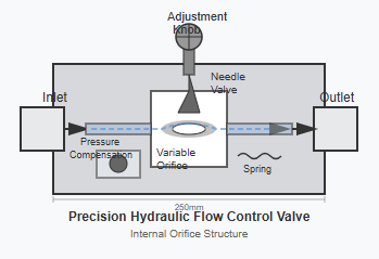
In hydraulic transmission systems, the hydraulic flow control valve plays a crucial role in regulating fluid flow through small orifices or clearances to achieve precise control of flow rate and pressure. This fundamental principle enables effective speed regulation and pressure adjustment in hydraulic systems.
The leakage phenomena in hydraulic components also falls under the category of clearance flow dynamics. Therefore, studying the flow calculation methods for orifices and clearances, along with understanding their influencing factors, is essential for the rational design of hydraulic systems and accurate analysis of the working performance of hydraulic components and systems.
Orifices in a hydraulic flow control valve can be classified into three distinct categories based on their length-to-diameter ratio (l/d):
When l/d ≤ 0.5
When l/d > 4
When 0.5 < l/d ≤ 4
Each type exhibits different flow characteristics that directly impact the performance of the hydraulic flow control valve in various applications.
Let us first examine the flow calculation for thin-walled orifices, which are commonly found in precision hydraulic flow control valve designs. Figure 2-16 illustrates a typical thin-walled orifice with a sharp-edged inlet configuration.
Due to inertial effects, the liquid flow undergoes contraction when passing through the orifice, creating a vena contracta - the minimum cross-sectional area of the flow stream - located slightly downstream of the orifice.
For thin-walled circular orifices, when the ratio of the upstream channel diameter to the orifice diameter (d₁/d) is greater than or equal to 7, the flow contraction is not influenced by the inner walls of the upstream channel. This condition is termed "complete contraction." Conversely, when d₁/d < 7, the upstream channel provides a guiding effect for the flow entering the orifice, resulting in "incomplete contraction."
Comparison of flow characteristics across different orifice types
Applying Bernoulli's equation between the upstream cross-section 1-1 and the downstream cross-section 2-2 of the hydraulic flow control valve orifice:
frac{p_1}{\rho} + \frac{\alpha_1 v_1^2}{2} + h_1 g = \frac{p_2}{\rho} + \frac{\alpha_2 v_2^2}{2} + h_2 g + h_w g
Where:
These losses can be expressed as:
h_{w1} = \zeta \frac{v_e^2}{2g}, \quad h_{w2} = \left(1 - \frac{A_e}{A_2}\right)\frac{v_e^2}{2g}
Since A_e ≤ A_2, the total energy loss becomes:
h_w = h_{w1} + h_{w2} = \zeta \frac{v_e^2}{2g} + \left(1 - \frac{A_e}{A_2}\right)\frac{v_e^2}{2g} = (\zeta + 1)\frac{v_e^2}{2g}
Substituting into the Bernoulli equation and noting that A₁ = A₂ (hence v₁ = v₂, α₁ = α₂) and h₁ = h₂, we obtain:
v_e = \frac{1}{\sqrt{1 + \zeta}} \sqrt{\frac{2}{\rho}(p_1 - p_2)} = C_v \sqrt{\frac{2}{\rho}\Delta p}
Where:
The flow rate through a thin-walled orifice in a hydraulic flow control valve is:
q = A_e v_e = C_v C_c A_T \sqrt{\frac{2}{\rho}\Delta p} = C_q A_T \sqrt{\frac{2}{\rho}\Delta p} \quad (2-35)
Where:
The values of C_c, C_v, and C_q are determined experimentally.
| Condition | C_c (Contraction) | C_v (Velocity) | C_q (Flow) |
|---|---|---|---|
| Complete contraction (d₁/d ≥ 7) | 0.61 to 0.63 | 0.97 to 0.98 | 0.60 to 0.62 |
| Incomplete contraction (d₁/d < 7) | - | - | 0.70 to 0.80 |
| Short orifices | - | - | 0.82 |
Thin-walled orifices in a hydraulic flow control valve exhibit minimal sensitivity to temperature variations due to their short flow path, resulting in stable flow characteristics. This makes them ideal for throttling applications.
Flow through short orifices can be calculated using the thin-walled orifice formula, but with a different flow coefficient, typically C_q = 0.82. Short orifices are easier to manufacture than thin-walled orifices, making them suitable for fixed restrictor applications in hydraulic flow control valve assemblies.
For long orifices, the flow is predominantly laminar due to viscous effects. The flow calculation employs the circular pipe laminar flow formula (Equation 2-28):
q = \frac{\pi d^4 \Delta p}{128\mu l}
Unlike thin-walled orifices, long orifice flow rates are viscosity-dependent. Temperature changes affect oil viscosity, consequently altering the flow rate - a characteristic significantly different from thin-walled orifice behavior.
The various orifice flow formulas can be consolidated into a universal equation applicable to any hydraulic flow control valve:
q = K A_T \Delta p^m \quad (2-36)
Where:
This universal formula (2-36) is frequently employed to analyze the flow-pressure characteristics of hydraulic flow control valve systems.
In hydraulic devices, clearances (or gaps) exist between various components, particularly between parts with relative motion. Oil flow through these clearances results in leakage, termed clearance flow. Due to the narrow nature of clearance channels, wall effects dominate, resulting in laminar flow conditions.
Clearance flow in hydraulic flow control valve assemblies occurs in two modes:
These two flow modes often coexist in practical applications.
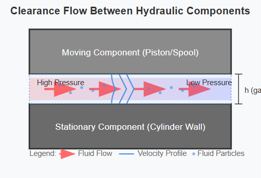
Parallel plate clearances can be formed between either fixed or relatively moving parallel plates, both common configurations in hydraulic flow control valve designs.
Consider the fixed parallel plate clearance flow illustrated in Figure 2-17. Let the clearance thickness be δ, width be b, length be l, with pressures p₁ and p₂ at the two ends. Extracting an infinitesimal parallelepiped element (volume b·dx·dy) from the clearance, with pressures p and (p + dp) on the left and right faces, and shear stresses (τ + dτ) and τ on the upper and lower surfaces, the force equilibrium equation is:
p \cdot b \cdot dy + (\tau + d\tau) \cdot b \cdot dx = (p + dp) \cdot b \cdot dy + \tau \cdot b \cdot dx
Simplifying yields:
frac{d\tau}{dy} = \frac{dp}{dx}
Since τ = μ(du/dy), the equation becomes:
frac{d^2u}{dy^2} = \frac{1}{\mu}\frac{dp}{dx}
Integrating twice with respect to y:
u = \frac{1}{2\mu}\frac{dp}{dx}y^2 + C_1y + C_2 \quad (2-37)
Where C₁ and C₂ are integration constants. Applying boundary conditions u = 0 at y = 0 and y = δ:
C_1 = -\frac{\delta}{2\mu}\frac{dp}{dx}, \quad C_2 = 0
In clearance flow, the pressure gradient dp/dx is constant:
frac{dp}{dx} = \frac{p_2 - p_1}{l} = -\frac{\Delta p}{l}
Substituting into equation (2-37):
u = \frac{\Delta p}{2\mu l}(\delta - y)y
The flow rate through fixed parallel plate clearances under pressure-driven flow in a hydraulic flow control valve is:
q = \int_0^\delta u \cdot b \cdot dy = \frac{b\delta^3}{12\mu l}\Delta p \quad (2-39)
Equation (2-39) reveals that pressure-driven flow through fixed parallel plate clearances is proportional to the cube of clearance thickness δ, indicating the significant impact of clearance size on leakage in hydraulic components.
As shown in Figure 2-2, when one plate is fixed and the other moves with velocity u₀, viscous effects cause the oil adjacent to the moving plate to travel at velocity u₀, while oil at the fixed plate remains stationary. The intermediate fluid layers exhibit a linear velocity distribution, characteristic of shear flow. With an average fluid velocity v = u₀/2, the flow rate due to plate relative motion is:
q' = vA = \frac{1}{2}u_0 b\delta \quad (2-40)
Equation (2-40) represents the shear-driven flow rate through parallel plate clearances.
In general applications within a hydraulic flow control valve, moving parallel plate clearances experience both pressure-driven and shear-driven flows. The total flow rate is the algebraic sum of both components:
q = \frac{b\delta^3}{12\mu l}\Delta p \pm \frac{1}{2}u_0 b\delta \quad (2-41)
Where u₀ represents the relative velocity between parallel plates. The positive sign applies when the direction of long plate motion relative to the short plate aligns with the pressure differential direction; the negative sign applies for opposite directions.
In hydraulic components such as the piston-cylinder interface in hydraulic cylinders and the spool-bore interface in hydraulic flow control valve assemblies, annular clearances are prevalent. These clearances exist in both concentric and eccentric configurations, each with distinct flow formulas.
Concentric annular clearance flow visualization
Eccentric annular clearance flow visualization
Figure 2-18 illustrates flow through a concentric annular clearance. With cylinder diameter d, clearance thickness δ, and clearance length l, if the annular clearance is "unwrapped" circumferentially, it becomes equivalent to a parallel plate clearance. Therefore, by substituting πd for b in equation (2-41), we obtain the flow formula for concentric annular clearances with relative motion between inner and outer surfaces:
q = \frac{\pi d\delta^3}{12\mu l}\Delta p \pm \frac{1}{2}\pi d\delta u_0 \quad (2-42)
When relative velocity u₀ = 0, this reduces to the formula for stationary concentric annular clearances:
q = \frac{\pi d\delta^3}{12\mu l}\Delta p \quad (2-43)
When the inner and outer circles are not concentric, with eccentricity e (Figure 2-19), an eccentric annular clearance forms. The flow formula for this configuration in a hydraulic flow control valve becomes:
q = \frac{\pi d\delta^3}{12\mu l}\Delta p (1 + 1.5\varepsilon^2) \pm \frac{1}{2}\pi d\delta u_0 \quad (2-44)
Where:
From equation (2-44), when ε = 0, it reduces to the concentric annular clearance formula. When ε = 1 (maximum eccentricity), the pressure-driven flow becomes 2.5 times that of the concentric configuration. This demonstrates that maintaining concentricity between mating components in hydraulic flow control valve designs is crucial for minimizing clearance leakage.
The temperature sensitivity of different orifice types in a hydraulic flow control valve varies significantly. Thin-walled orifices maintain relatively stable flow characteristics across temperature ranges due to their minimal flow path length. This stability makes them preferred choices for precision throttling applications where consistent performance is critical.
In contrast, long orifices exhibit substantial temperature dependence because viscosity changes directly affect laminar flow conditions. Engineers must account for these variations when designing hydraulic flow control valve systems operating across wide temperature ranges. Temperature compensation mechanisms may be necessary to maintain consistent system performance.
Flow rate variation with temperature for different orifice types
The cubic relationship between clearance thickness and leakage flow (as shown in equations 2-39 and 2-43) emphasizes the critical importance of manufacturing precision in hydraulic flow control valve components. Even minor variations in clearance dimensions can result in significant changes in leakage rates.
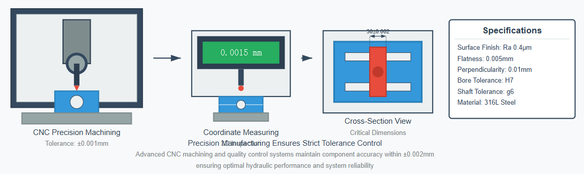
Modern manufacturing techniques such as precision grinding, honing, and lapping are employed to achieve the tight tolerances required for optimal performance.
When designing a hydraulic flow control valve, engineers must balance multiple competing factors:
Thin-walled orifices provide the most stable flow characteristics but may be challenging to manufacture consistently.
Short orifices offer a good compromise between performance and manufacturability, making them suitable for many fixed restrictor applications.
Maintaining concentricity in annular clearances is essential. Design features such as pressure balancing and proper bearing support help maintain alignment during operation.
The choice between different orifice types affects system response time. Thin-walled orifices typically provide faster response due to their lower flow inertia.
Modern hydraulic flow control valve designs often incorporate sophisticated features to enhance performance:
Allow real-time adjustment of flow characteristics to match changing system requirements. These may include needle valves, spool valves, or poppet valves with precisely controlled positioning systems.
Combining different orifice types in series or parallel configurations enables more complex flow-pressure relationships, expanding the operational envelope of the hydraulic flow control valve.
Incorporating pressure-compensating elements maintains constant flow rates despite variations in system pressure, essential for many industrial applications.
Integration of flow sensors with electronic control systems enables closed-loop control of hydraulic flow control valve operation, improving accuracy and repeatability.
The small clearances and orifices in a hydraulic flow control valve make them particularly sensitive to contamination. Particles comparable in size to clearance dimensions can cause blockage, erosion, or jamming.
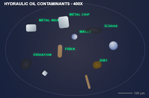
Microscopic view of hydraulic fluid contaminants that can affect valve performance
Proper filtration is essential, with filter ratings typically specified at levels significantly smaller than the minimum clearance dimensions. In critical applications, multi-stage filtration systems may be employed to ensure fluid cleanliness.
High-velocity flow through orifices can lead to cavitation, particularly when large pressure drops occur. This phenomenon can cause erosion damage, noise, and performance degradation in hydraulic flow control valve components.
The interaction between flow forces and mechanical elements in a hydraulic flow control valve can lead to dynamic instabilities such as oscillation or hunting. Understanding these phenomena requires consideration of:
The principles governing flow through orifices and clearances form the foundation for understanding and designing effective hydraulic flow control valve systems. From the basic flow equations for thin-walled, short, and long orifices to the complex interactions in eccentric annular clearances, each configuration offers unique characteristics that can be leveraged for specific applications.
The universal flow formula provides a unified framework for analyzing different orifice types, while the detailed examination of clearance flows reveals the critical importance of manufacturing precision and alignment in minimizing leakage. Temperature effects, contamination sensitivity, and dynamic behavior all play crucial roles in determining overall system performance.
As hydraulic systems continue to evolve toward higher pressures, greater precision, and improved efficiency, the fundamental understanding of flow through orifices and clearances remains essential. Modern hydraulic flow control valve designs incorporate these principles with advanced materials, manufacturing techniques, and control strategies to meet increasingly demanding performance requirements.
Engineers designing hydraulic systems must carefully consider the trade-offs between different orifice and clearance configurations, accounting for factors such as flow stability, temperature sensitivity, manufacturing feasibility, and long-term reliability. By applying these fundamental principles with modern analytical and design tools, optimal hydraulic flow control valve solutions can be developed for a wide range of industrial, mobile, and aerospace applications.
The continued advancement of hydraulic technology relies on both theoretical understanding and practical application of these flow principles. As new materials, manufacturing processes, and control technologies emerge, the basic relationships described in this article will continue to guide the development of next-generation hydraulic flow control valve systems that are more efficient, precise, and reliable than ever before.