
Real liquids possess viscosity, which creates resistance during flow. To overcome this resistance, flowing liquids must expend a portion of their energy. This energy loss is represented by the term hw·g in the actual liquid Bernoulli equation, as shown in equation (2-23). When this term is converted to pressure loss, it can be expressed as Δp = ρghw. In hydraulic systems equipped with a hydraulic pressure relief valve, these pressure losses convert hydraulic energy into thermal energy, leading to increased system temperatures. Therefore, when designing hydraulic systems, minimizing pressure losses becomes crucial for optimal performance.
Pressure losses can be categorized into two main types: losses along the pipe length and local pressure losses. Let's examine the calculation methods for each type in detail.
Pressure loss in hydraulic systems directly impacts energy efficiency and system performance. A properly sized hydraulic pressure relief valve must account for these losses to ensure accurate pressure control and system protection.
When liquid flows through a constant-diameter straight pipe, viscous friction creates what we call pressure loss along the pipe length. Different flow states of the liquid produce varying degrees of pressure loss along the pipe. Understanding these losses is essential for proper hydraulic pressure relief valve selection and system design.
During laminar flow, liquid particles move in an orderly pattern, allowing us to use mathematical tools to comprehensively explore flow conditions and ultimately derive formulas for calculating pressure losses along the pipe.
In Figure 2-14, liquid flows through a constant-diameter horizontal straight pipe in laminar flow state. Consider a small cylindrical element aligned with the pipe axis as our research object. With radius r and length l, pressures p₁ and p₂ act on its two end faces, while internal friction force Ff acts on its lateral surface. When the liquid flow moves at constant velocity, it's in force equilibrium, hence:
(p₁ - p₂)πr² = Ff
The friction force can be expressed as:
Ff = -2πrlμ(du/dr)
The negative sign indicates that flow velocity u decreases as r increases. If we let Δp = p₁ - p₂, substituting Ff into the equation and rearranging gives:
du = -(Δp/2μl)r dr
Integrating this expression and applying boundary conditions (when r = R, u = 0), we obtain:
u = (Δp/4μl)(R² - r²) ... (2-27)
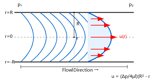
Figure 2-14: Velocity distribution in laminar pipe flow follows a parabolic profile
This shows that the flow velocity of liquid particles in the pipe follows a parabolic distribution in the radial direction. The minimum velocity occurs at the pipe wall (r = R) where umin = 0, while the maximum velocity occurs at the pipe axis (r = 0) where:
umax = (Δp/4μl)R² = (Δp/16μl)d²
For a small annular cross-section with radius r and width dr, the area is dA = 2πr dr, and the flow rate through it is:
dq = u dA = 2πu r dr = 2π(Δp/4μl)(R² - r²)r dr
Integrating yields:
q = ∫₀ᴿ 2π(Δp/4μl)(R² - r²)r dr = (πR⁴/8μl)Δp = (πd⁴/128μl)Δp ... (2-28)
This fundamental equation is crucial for determining flow rates in systems with a hydraulic pressure relief valve.
Based on the definition of average velocity:
v = q/A = (1/(πd²/4)) · (πd⁴/128μl)Δp = (d²/32μl)Δp ... (2-29)
Comparing equation (2-29) with umax shows that the average velocity v equals half of the maximum velocity umax.
Rearranging equation (2-29) gives the pressure loss along the pipe as:
Δpλ = Δp = (32μlv/d²)
This equation reveals that for laminar flow in straight pipes, pressure loss is directly proportional to pipe length, flow velocity, and viscosity, while being inversely proportional to the square of the pipe diameter. These relationships are critical when sizing a hydraulic pressure relief valve for system protection.
By appropriately transforming the equation, the pressure loss calculation formula can be rewritten as:
Δpλ = (64ν/dv) · (l/d) · (ρv²/2) = (64/Re) · (l/d) · (ρv²/2) = λ · (l/d) · (ρv²/2) ... (2-30)
Where λ is the resistance coefficient along the pipe. For circular pipe laminar flow, the theoretical value is λ = 64/Re. Considering that actual circular pipe cross-sections may deform and liquid layers near the pipe wall may cool, practical calculations use λ = 75/Re for metal pipes and λ = 80/Re for rubber hoses.
Equation (2-30) was derived under horizontal pipe conditions. Since pressure changes caused by liquid weight and position changes are minimal and negligible, this formula also applies to non-horizontal pipes.
The formula for calculating pressure loss along the pipe during turbulent flow has the same form as for laminar flow:
Δpλ = λ(l/d) · (ρv²/2)
However, the resistance coefficient λ depends not only on Reynolds number Re but also on pipe wall roughness: λ = f(Re, Δ/d), where Δ is the absolute roughness of the pipe wall, and the ratio Δ/d is called the relative roughness.
For smooth pipes: λ = 0.3164Re(-0.25)
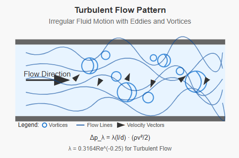
Figure 2-15: Turbulent flow characteristics showing irregular fluid motion
For rough pipes, λ values can be found from relevant curves in handbooks based on different Re and Δ/d values. When installing a hydraulic pressure relief valve, these roughness factors must be considered to ensure accurate pressure settings.
When liquid flows through pipe bends, pipe joints, sudden cross-section changes, valve ports, filters, and other local devices, the flow creates vortices and intense turbulence phenomena. The resulting pressure losses are called local pressure losses. When liquid passes through these various local devices, flow conditions become extremely complex with numerous influencing factors. Local pressure loss values are difficult to analyze theoretically, so resistance coefficients for local pressure losses must generally be determined experimentally.
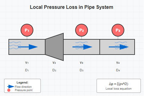
Figure 2-16: Examples of components causing local pressure losses
The calculation formula for local pressure losses is:
Δpζ = ζ(ρv²/2) ... (2-31)
Where ζ is the local resistance coefficient. Values of ζ for various local device structures can be found in relevant handbooks. Understanding these losses is essential when positioning a hydraulic pressure relief valve in the system.
Local pressure losses for liquid flowing through various valves can also be calculated using equation (2-31). However, due to the complex internal channel structures of valves, calculations using this formula are difficult. Therefore, the practical calculation formula for local pressure losses Δpv through valve components is:
Δpv = Δpn(q/qn)² ... (2-32)
The total pressure loss of an entire pipeline system equals the sum of all pressure losses along the pipe and all local pressure losses:
ΣΔp = ΣΔpλ + ΣΔpζ + ΣΔpv = Σλ(l/d)·(ρv²/2) + Σζ(ρv²/2) + ΣΔpn(q/qn)² ... (2-33)
In hydraulic systems, the vast majority of pressure losses convert to thermal energy, causing system temperature increases, increased leakage, and ultimately affecting system performance. A properly sized hydraulic pressure relief valve helps manage these pressure variations and protects the system from excessive pressures.
From the pressure loss calculation formulas, we can see that reducing flow velocity, shortening pipeline length, minimizing sudden cross-section changes, and improving the processing quality of inner pipe walls all contribute to reduced pressure losses. Among these factors, flow velocity has the greatest impact, so liquid velocity in pipeline systems should not be excessive. However, if the velocity is too low, it will increase the size of pipes and valve components, thereby increasing costs.
In the hydraulic system shown in Figure 2-15, given:
Required:
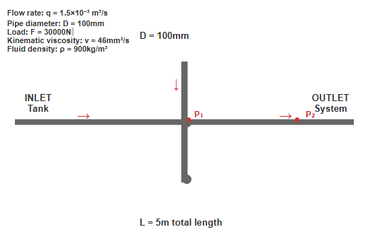
Figure 2-17: Schematic of the hydraulic system in Example 2-4
(1) Calculate inlet path pressure loss:
Inlet pipe flow velocity:
v₁ = q/(π/4·d²) = 1.5×10⁻³/(π/4×(20×10⁻³)²) m/s = 4.77 m/s
Reynolds number:
Re = v₁d/ν = 4.77×20×10⁻³/46×10⁻⁶ = 2074 < 2320 (laminar flow)
Resistance coefficient along the pipe:
λ = 75/Re = 75/2074 = 0.036
Therefore, inlet path pressure loss:
ΣΔp = λ(l/d)·(ρv₁²/2) + Σζ(ρv₁²/2)
= (0.036×5/20×10⁻³ + 7.2)×900×4.77²/2 Pa
= 0.166×10⁶ Pa = 0.166 MPa
(2) Calculate pump supply pressure:
Applying Bernoulli's equation between pump outlet section 1-1 and hydraulic cylinder inlet section 2-2:
p₁ + ρgh₁ + ½ρα₁v₁² = p₂ + ρgh₂ + ½ρα₂v₂² + Δp_w
Rearranging for p₁:
p₁ = p₂ + ρg(h₂ - h₁) + ½ρ(α₂v₂² - α₁v₁²) + Δp_w
Where:
Therefore, pump supply pressure:
p₁ = (3.81 + 0.044 - 0.02 + 0.166) MPa = 4 MPa
This calculation demonstrates why a hydraulic pressure relief valve must be carefully selected to handle the system's operating pressures while accounting for all pressure losses.
From this example's calculation of p₁, we observe that in hydraulic transmission systems, pressure changes caused by liquid position height variations and flow velocity changes are relatively small. In general calculations, the terms ρg(h₂ - h₁) and ½ρ(α₂v₂² - α₁v₁²) can be neglected. Therefore, the expression for p₁ can be simplified to:
p₁ = p₂ + ΣΔp ... (2-34)
Although equation (2-34) is an approximation, it has gained widespread application in hydraulic system design calculations. This simplified approach is particularly useful when determining the setting pressure for a hydraulic pressure relief valve.
As pressure losses convert to thermal energy, system temperature rises affect fluid viscosity, which in turn influences pressure losses. This creates a complex feedback loop that must be considered in system design. The hydraulic pressure relief valve plays a crucial role in managing these thermal effects by limiting maximum system pressures and preventing excessive heat generation.
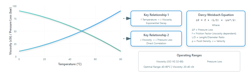
Figure 2-18: Relationship between temperature, viscosity, and pressure loss in hydraulic systems
To minimize pressure losses in hydraulic systems:
Select appropriate pipe diameters based on flow requirements and acceptable pressure losses. Larger diameters reduce velocity and pressure losses but increase system cost and size.
Minimize the number of bends, joints, and sudden cross-section changes. Use gradual transitions where diameter changes are necessary.
Specify appropriate internal surface finishes for pipes and components. Smoother surfaces reduce friction losses, particularly important in high-flow applications.
Choose valves and fittings with low pressure drop characteristics. The hydraulic pressure relief valve should be selected not only for its pressure setting range but also for its flow capacity and pressure drop characteristics.
The hydraulic pressure relief valve serves as a critical safety component, protecting the system from overpressure conditions that could result from:
Proper sizing and setting of the hydraulic pressure relief valve requires comprehensive understanding of all pressure losses in the system, including both normal operating conditions and potential failure modes.
When implementing these principles in actual hydraulic system design:
Include appropriate safety factors when calculating total system pressure requirements. The hydraulic pressure relief valve setting should typically be 10-15% above maximum operating pressure but well below component pressure ratings.
Consider the dynamic behavior of pressure losses during transient conditions such as startup, shutdown, and load changes. The hydraulic pressure relief valve must respond quickly enough to prevent pressure spikes.
Account for increased pressure losses over time due to contamination, wear, and degradation of system components. Regular maintenance and monitoring ensure the hydraulic pressure relief valve continues to protect the system effectively.
Understanding pressure losses in hydraulic systems is fundamental to proper system design and component selection. The mathematical relationships presented here provide the foundation for calculating both laminar and turbulent flow losses, as well as local losses through various system components. These calculations directly influence the selection and setting of the hydraulic pressure relief valve, which serves as both a system protector and a performance optimizer. By carefully considering all sources of pressure loss and implementing appropriate design strategies, engineers can create efficient, reliable hydraulic systems that operate safely within their design parameters while minimizing energy consumption and heat generation.
The hydraulic pressure relief valve is a critical component that must be selected based on a comprehensive analysis of all system pressure losses. Proper calculation of both frictional and local losses ensures the valve will function correctly under all operating conditions, protecting system components while maintaining efficient operation.
Pressure loss calculations should account for flow regime (laminar vs. turbulent), pipe characteristics, component geometry, and operating conditions to ensure accurate hydraulic system design.